Hardening soil
The Hardening soil model introduced by Schanz et al. [1] is suitable for the modeling of a large group soft soils. The model combines two hardening mechanisms. The shear hardening mechanism drives the evolution of plastic strains caused by deviatoric stress components, while the compressive mechanism becomes active in the compressive mode of loading, e.g., in oedometer or in isotropic compression. The shear hardening mechanism is manifested by a gradual evolution of the shear yield surface fsHS in dependence on the current value of equivalent devitoric plastis strain κs(or γps).
This hardening process (yield surface expansion) is accompanied by the evolution of the mobilized angle of internal friction φm and is terminated by arriving at the limit shear yield surface fsMN. In the GEO5 FEM program this yield function is presented in the form of Matsuoka-Nakai failure criterion being the function of the peak values of shear strength parameters, the cohesion c, and the angle of internal friction φ. The projection of the yield surface into the deviatoric plane is therefore a smooth convex curve passing through all vertexes of the Mohr-Coulomb model. The consequence of compressive hardening is an evolution of the cap yield surface fcHS in dependence on the evolution of preconsolidation pressure pc. A similar formulation developed in terms of invariant stress measures was also presented in [2].
A graphical representation of both yield surfaces is evident from the following figure. A gradual evolution of the shear yield surface, evident from the projection of the yield surface into the meridian plane plane, is presented for illustration. In a similar fashion is defined the Soft soil model, which, however, implements the limit shear surface only. The hardening is therefore limited to the compressive cap.
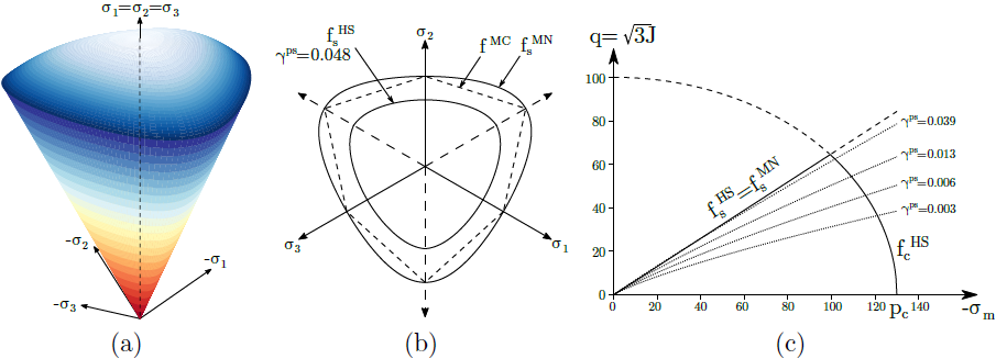 a) yield surface in principal stress space, b) projection into deviatoric and c) meridian planes
Formulation of the shear yield surface arises from the assumption that the relationship between the deviatoric stress q and vertical strain ε3 during drained triaxial test can be described by a hyperbolic function. The corresponding stress-strain diagram is shown in the following figure, where qa is the asymptotic value of q and qfMC corresponds to the value of q when reaching the limit surface in which case it holds qf = Rfqa, where Rf is the reduction coefficient. Further details can be found in the theoretical manual.
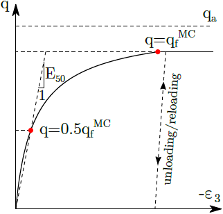 Hyperbolic stress-strain law
Parameters defining the Hardening soil material model are summarized in the following table.
Symbol | Units | Description | |
| [MPa] | Secant modulus of elasticity | |
| [MPa] | Modulus of unloading/reloading | |
| [-] | Poisson's ratio | |
| [kPa] | Reference mean stress | |
| [-] | Exponent of stiffness power law | |
| [kPa] | Limit value of mean stress to ensure non-zero stiffness | |
| [kN/m3] | Bulk weight | |
| [-] | Initial void ratio corresponding to the state at the end of 1st calculation stage | |
| [-] | Failure ratio | |
| [kPa] | Peak effective cohesion | |
| [°] | Peak effective angle of internal friction | |
| [°] | Dilatancy angle | |
| Bulk weight | ||
| [-] | Coefficient of lateral earth pressure at rest of normally consolidated soil | |
| [MPa] | Tangent edometric modulus | |
| [kPa] | Reference vertical stress to determine | |
| [-] | Maximum void ratio to terminate dilation (when limiting dilation) | |
| [-] | Overconsolidation ratio | |
| [kPa] | Preoverburden pressure | |
| [1/K] | Coefficient of thermal expansion (when considering temperature effects) | |
| [-] | Parameter defining the shape of compressive cap | |
| [Pa] | Hardening modulus (not inputted) | |
| [kPa] | Preconsolidation pressure | |
| [°] | Critical state friction angle (not inputted) | |
| [°] | Mobilized angle of internal friction (not inputted) | |
| [°] | Mobilized dilatancy angle (not inputted) |
The secant modulus of elasticity Eip,ref can be approximated with the help of the modulus of elasticity E50p,ref as follows
![]()
where index (p,ref) represents a reference value of the modulus pertinent to a certain reference value of the effective mean stress σmref. In general, the model assumes evolution of the modulus of elasticity as a function of the current mean stress in the form
![]()
Point out that this formulation differs from the one used for example in publications [1] and [2], where the evolution of stiffness depends on the minimum principal stress, here σ1. This should be taken into account when adopting parameters calibrated for a different engineering software in the GEO5 FEM program. A potential option is to use a modified set of parameters which yield a reasonable match of simulations provided by individual softwares. To this end, a simple linear regression appears sufficient to adjust parameters Eurp,ref and mp. An illustrative example of this particular approach is presented in the following figure.
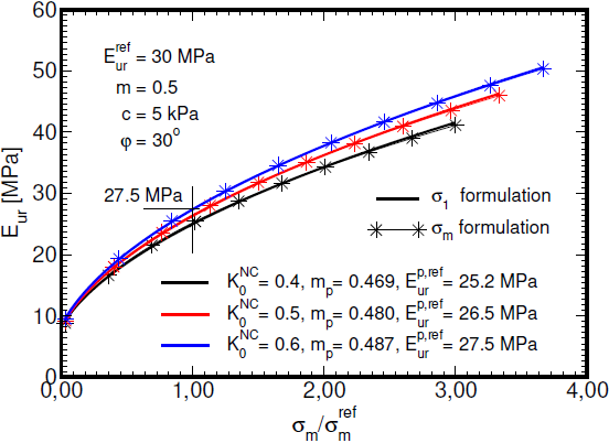 Determining dependence of modulus of unloading/reloading Eur on mean stress σm using linear regression
The modified parameters E50p,ref(Eip,ref) and Rf can obtained subsequently within an optimization step by comparing numerical simulations of a triaxial compression test while exploiting already determined parameters Eurp,ref a mp.
Details can be found in the theoretical manual. However, it is strongly recommended to calibrate the specific model parameters, linked to a particular implementation, from the provided laboratory measurements employing for example the calibration software ExCalibre.
The compression cap fcHS is characterized by the parameter M determining its shape and by the hardening modulus H providing the increment of preconsolidation pressure Δpc in terms of the increment of volumetric plastic strain Δεvpl. The hardening modulus H is given by
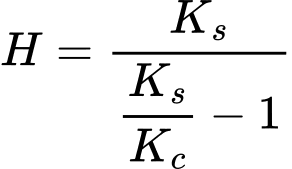
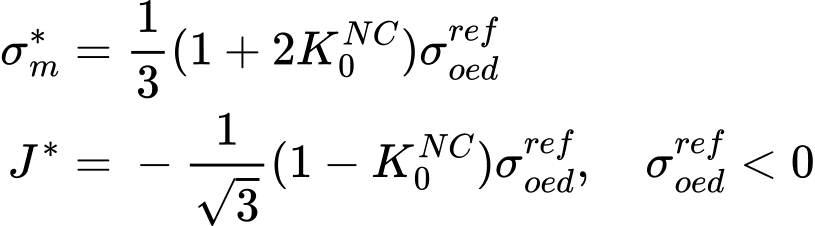
where Kc, Ks are the bulk moduli at primary loading and unloading, respectively. Further details are available in the theoretical manual. The parameters ![]() can be either directly inputted or determined automatically based on the values of the coefficient of lateral earth pressure at rest for normally consolidated soils K0NC and oedometric modulus Eoedref. This is accomplished using numerical optimization of an oedometric laboratory test. The objective is to determined model parameters M, H such that the numerically predicted oedometric modulus matches the one specified for a given value of K0NC as evident from the following figure. The mean stress σm* and equivalent deviatoric stress J* are given by
can be either directly inputted or determined automatically based on the values of the coefficient of lateral earth pressure at rest for normally consolidated soils K0NC and oedometric modulus Eoedref. This is accomplished using numerical optimization of an oedometric laboratory test. The objective is to determined model parameters M, H such that the numerically predicted oedometric modulus matches the one specified for a given value of K0NC as evident from the following figure. The mean stress σm* and equivalent deviatoric stress J* are given by
Further details can be found in the theoretical manual.
 a) graphical representation of reference oedometric modulus Eoedref at a point of specified σoedref, b) current stress at the end of optimization step associated with σoedref
The Hardening soil model allows for the modeling of soil dilation (evolution of positive volumetric plastic strains during plastic shearing) by introducing the
dilatancy angle ψ. The evolution of plastic strains is driven by plastic potential gsHS. Definition of plastic potential is essentially identical to that adopted for the Drucker-Prager model. The only difference is seen in the definition of the slope of plastic potential Mψ which now depends on the current value of the mobilized angle of internal friction ψm. The corresponding evolution equation builds, similarly to the Modified Mohr-Coulomb model, on the Rowe dilation theory
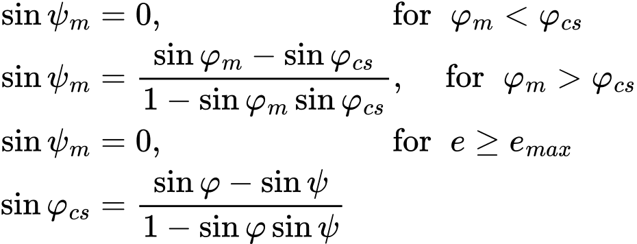
where φ, φm, φcs, ψ are the peak angle of internal friction, the mobilized angle of internal friction, the critical state friction angle, and the peak dilatancy angle. A graphical representation of the evolution of ψm is evident from the following figure. It also illustrates a potential dilatancy cutoff by introducing the maximum void ratio emax, for which reaching the critical state ψm = 0 is expected.
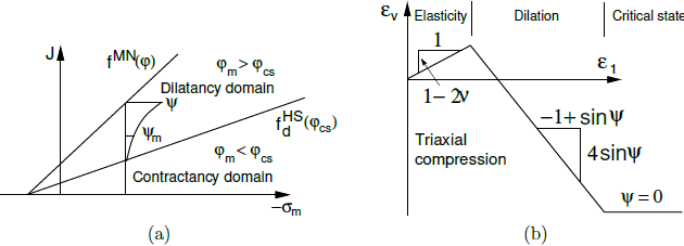 Rowe dilation theory: a) graphical representation of evolution of mobilized dilatancy angle ψm, b) dilatancy cutoff
Recall that the stiffness evolution depends on the current value of the mean effective stress σm. This is closely related to the selection of the initial load step, which requires for very low values of initial stress to be sufficiently small. To speed up convergence it appears useful to exploit the Minimum number of iterations for a single load step. The influence of magnitude of the initial load step on the evolution of stress and strain is described in detail here.
An important step in light of a successful analysis is associated with setting the initial values of the preconsolidation stress pcin and equivalent plastic deviatoric strain κsin. Both parameters are set in dependence on the current stress state at the time the Hardening soil model is introduced into the analysis such that the current stress state satisfies both the shear and cap yield functions. Details are provided here. It is also possible to consult the description provided for the Modified Cam clay model.
The model allows for adjusting the initial value of preconsolidation pressure in dependence on the expected degree of preconsolidation by using parameters ![]() and
and ![]() . Details can be found here. Point out that this option is available only when setting the initial geostatic stress with the help of K0 procedure.
. Details can be found here. Point out that this option is available only when setting the initial geostatic stress with the help of K0 procedure.
Providing the undrained conditions are required in the analysis one may proceed with the Type (1): analysis in effective stress (cef, φe) only.
The Hardening soil model also allows for performing the stability analysis. However, this option is available only when running the stability analysis analysis within a given construction stage. In such a case, the compression cap is turned off and similarly the evolution of the mobilized friction angle. Therefore, only the limit yield surface fsMN may become active. The task is solved by gradually reducing the peak shear strength parameters c, φ in the same way as outlined for the Drucker-Prager model.
The model performance in the framework of simple laboratory tests is examined here including the influence of magnitude of the initial load step.
Unless there is clear experimental evidence for different values, the parameters of the Hardening soil model should fit into the recommended ranges listed in the following table.
Symbol | Units | Recommended value | |
| [MPa] | (2, 70) | |
| [MPa] |
| |
| [kPa] | 100.0 | |
| [-] | (0.3, 0.9) | |
| [kPa] | 10.0 | |
| [-] | 0.9 | |
| [°] | (16.0, 42.0) | |
| [kPa] | (0.0, 50.0) | |
| [°] |
| |
| [-] | (0.5, 2.5) | |
| [-] | 0,2 | |
| [-] |
| |
| [-] |
| |
| [kPa] | 100.0 | |
| [MPa] |
|
Implementation of the Hardening soil material model into the GEO5 FEM program is described in detail in the theoretical manual.
Literature:
[1] T. Schanz, P.A. Vermeer, P.G. Bonnier, The hardening soil model: Formulation and verification, Beyond 2000 in Computational Geotechnics, Balkema, Rotterdam. 1999
[2] T. Benz, Small-Strain Stiffness of Soils and its Numerical Consequences, PhD thesis, University of Stuttgart, 2007